Apache Spark is a lightning-fast cluster computing technology, designed for fast computation. It is based on Hadoop MapReduce and it extends the MapReduce model to efficiently use it for more types of computations, which includes interactive queries and stream processing. The main feature of Spark is its in-memory cluster computing that increases the processing speed of an application.
Spark is designed to cover a wide range of workloads such as batch applications, iterative algorithms, interactive queries and streaming. Apart from supporting all these workload in a respective system, it reduces the management burden of maintaining separate tools.
Spark provides developers and engineers with a Scala API. The Spark tutorials with Scala listed below cover the Scala Spark API within Spark Core, Clustering, Spark SQL, Streaming, Machine Learning MLLib and more.
Apache Spark Components
Apache Spark puts the promise for faster data processing and easier development. How Spark achieves this? To answer this question, let’s introduce the Apache Spark ecosystem which is the important topic in Apache Spark introduction that makes Spark fast and reliable. These components of Spark resolves the issues that cropped up while using Hadoop MapReduce.
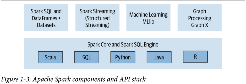
- Spark Core
It is the kernel of Spark, which provides an execution platform for all the Spark applications. It is a generalized platform to support a wide array of applications.
- Spark SQL
It enables users to run SQL/HQL queries on the top of Spark. Using Apache Spark SQL, we can process structured as well as semi-structured data. It also provides an engine for Hive to run unmodified queries up to 100 times faster on existing deployments.
- Spark Streaming
Apache Spark Streaming enables powerful interactive and data analytics application across live streaming data. The live streams are converted into micro-batches which are executed on top of spark core.
- Spark MLlib
It is the scalable machine learning library which delivers both efficiencies as well as the high-quality algorithm. Apache Spark MLlib is one of the hottest choices for Data Scientist due to its capability of in-memory data processing, which improves the performance of iterative algorithm drastically.
- Spark GraphX
Apache Spark GraphX is the graph computation engine built on top of spark that enables to process graph data at scale.
- SparkR
It is R package that gives light-weight frontend to use Apache Spark from R. It allows data scientists to analyze large datasets and interactively run jobs on them from the R shell. The main idea behind SparkR was to explore different techniques to integrate the usability of R with the scalability of Spark.
RDDs and Dataframes
There are 3 main data structures in Spark:
- RDDs
- Dataframes
- Data sets
These data structures in Spark help to store the extracted data until it is loaded into a data source after processing.
Everything in Spark is an RDD. Dataframes and data sets are also abstractions of RDD.
RDD
Resilient Distributed Dataset (RDD) is the fundamental unit of data in Apache Spark, which is a distributed collection of elements across cluster nodes and can perform parallel operations. Spark RDDs are immutable but can generate new RDD by transforming existing RDD.
When you load the data into a Spark application, it creates an RDD that stores the loaded data.
Spark gets the data file, splits it into small chunks of data, and distributes those chunks of data across the cluster. This collection of data is referred to as RDDs.
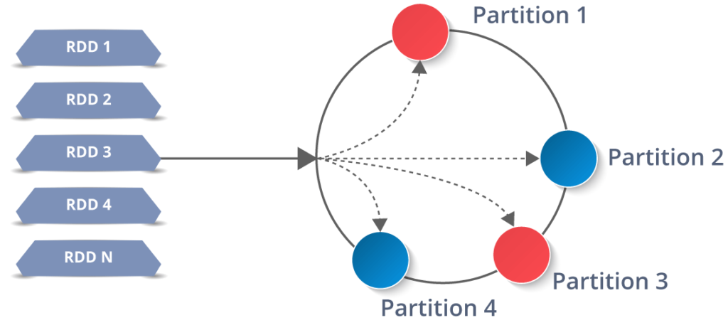
There are three ways to create RDDs in Spark:
- Parallelized collections – We can create parallelized collections by invoking parallelized method in the driver program.
- External datasets – By calling a textFile method one can create RDDs. This method takes URL of the file and reads it as a collection of lines.
- Existing RDDs – By applying transformation operation on existing RDDs we can create new RDD.
Transformation and Action functions:
- Transformations are used to transform data into another.
- Actions are used to collect the distributed transformed results and create non-distributed data
In simple terms, what a Spark application does is,
- It extracts the data from a data source and stores them in a data frame or in an RDD.
- Then it processes the data using transformation functions and collects the results using action functions.
- Then it loads the processed data again to a data source according to the requirement.
Spark Architecture
Apache Spark uses master-slave architecture.
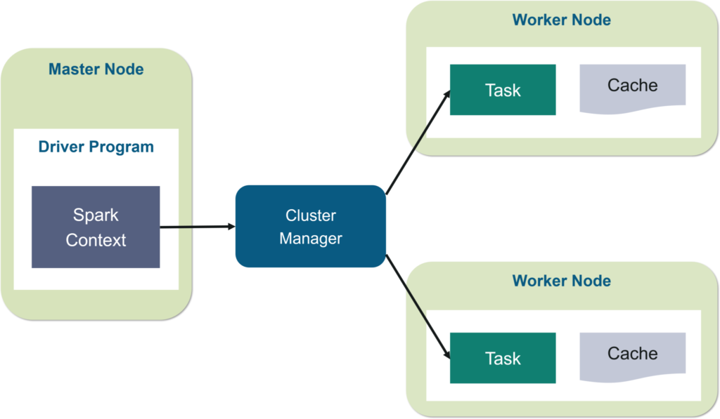
Just like in the real world, the master will get the job done by using his slaves. It means that you will have a master process and multiple slave processes which are controlled by that dedicated master process.
Master manages, maintains, and monitors the slaves while slaves are the actual workers who perform the processing tasks. You tell the master what wants to be done and the master will take care of the rest. It will complete the task, using its slaves.
In the Spark environment, master nodes are referred to as drivers, and slaves are referred to as executors.
Drivers: are the master process in the Spark environment. It contains all the metadata about slaves or, in Spark terms, executors. They are responsible for Analyzing, Distributing, Scheduling, and Monitoring the executors.
Executors: are the slave processes in the Spark environment. They perform the data processing which is assigned to them by their master.
Spark Application
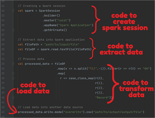
Spark application can be written in 3 steps. All you need is:
- Code to extract data from a data source.
- Code to process the extracted data.
- Code to load the data again into a data source.
On top of those three steps, we need a code to create a spark session in our application.
We know that when we apply to Spark, what Spark does is create a driver process, and that driver process executes our application using executors created by him.
Therefore, to create the connection between the driver process and our application, we need a spark session in our application.
Code structure might look as follows:
Spark Application and SparkSession
At the core of every Spark application is the Spark driver program, which creates a SparkSession object. When you’re working with a Spark shell, the driver is part of the shell and the SparkSession object (accessible via the variable spark) is created for you, as you saw in the earlier examples when you launched the shells.
In those examples, because you launched the Spark shell locally on your laptop, all the operations ran locally, in a single JVM. But you can just as easily launch a Spark shell to analyze data in parallel on a cluster as in local mode. The commands spark-shell –help or pyspark –help will show you how to connect to the Spark cluster man‐ ager. Figure 2-2 shows how Spark executes on a cluster once you’ve done this.
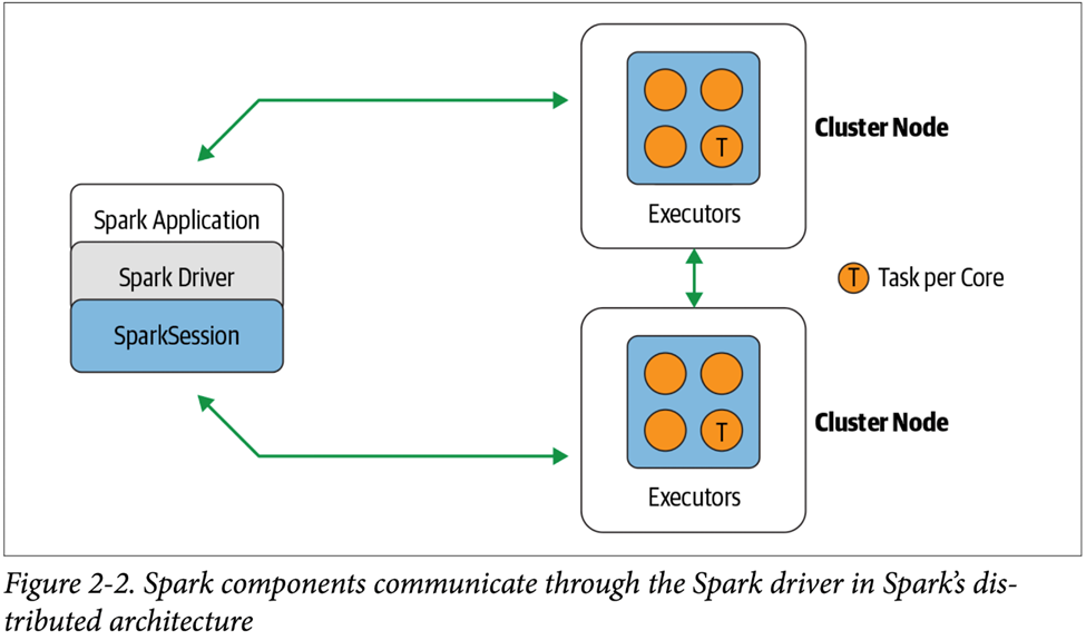
Once you have a SparkSession, you can program Spark using the APIs to perform Spark operations.
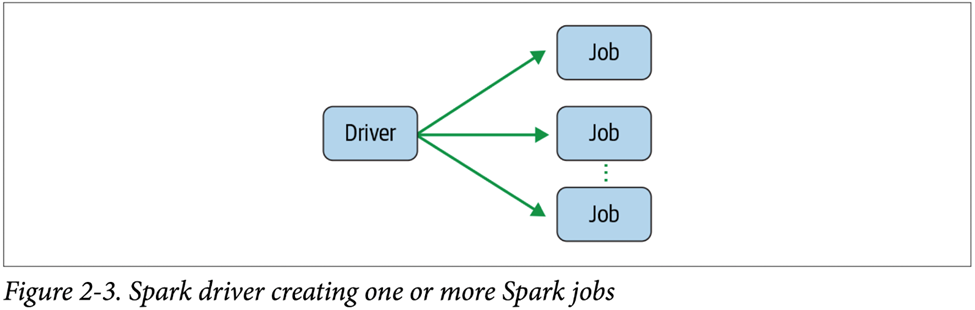
Spark Jobs
During interactive sessions with Spark shells, the driver converts your Spark application into one or more Spark jobs (Figure 2-3). It then transforms each job into a DAG. This, in essence, is Spark’s execution plan, where each node within a DAG could be a single or multiple Spark stages.
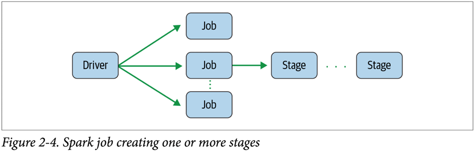
Spark Stage
As part of the DAG nodes, stages are created based on what operations can be per‐ formed serially or in parallel (Figure 2-4). Not all Spark operations can happen in a single stage, so they may be divided into multiple stages. Often stages are delineated on the operator’s computation boundaries, where they dictate data transfer among Spark executors.
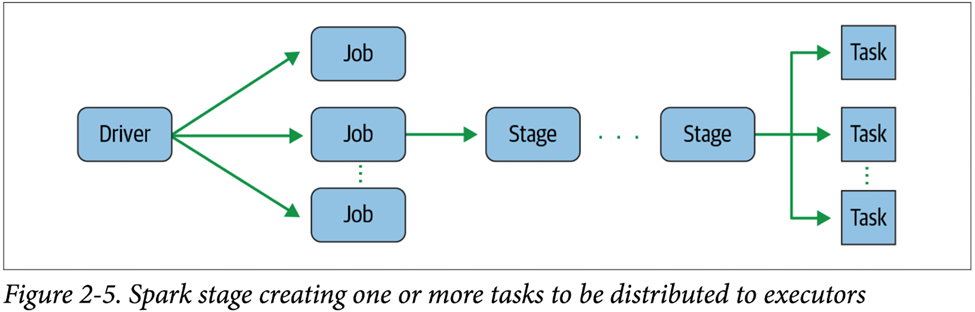
Spark Tasks
Each stage is comprised of Spark tasks (a unit of execution), which are then federated across each Spark executor; each task maps to a single core and works on a single par‐ tition of data (Figure 2-5). As such, an executor with 16 cores can have 16 or more tasks working on 16 or more partitions in parallel, making the execution of Spark’s tasks exceedingly parallel!
Transformations, Actions, and Lazy Evaluation
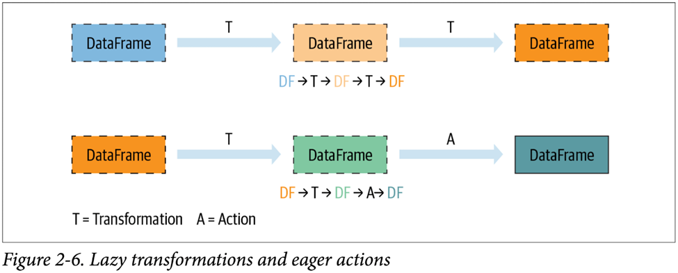
Spark operations on distributed data can be classified into two types: transformations and actions. Transformations, as the name suggests, transform a Spark DataFrame into a new DataFrame without altering the original data, giving it the property of immutability. Put another way, an operation such as select() or filter() will not change the original DataFrame; instead, it will return the transformed results of the operation as a new DataFrame.
All transformations are evaluated lazily. That is, their results are not computed immediately, but they are recorded or remembered as a lineage. A recorded lineage allows Spark, later in its execution plan, to rearrange certain transformations, coalesce them, or optimize transformations into stages for more efficient execution. Lazy evaluation is Spark’s strategy for delaying execution until an action is invoked or data is “touched” (read from or written to disk).
An action triggers the lazy evaluation of all the recorded transformations. In
Figure 2-6, all transformations T are recorded until the action A is invoked. Each transformation T produces a new DataFrame.
While lazy evaluation allows Spark to optimize your queries by peeking into your chained transformations, lineage and data immutability provide fault tolerance. Because Spark records each transformation in its lineage and the DataFrames are immutable between transformations, it can reproduce its original state by simply replaying the recorded lineage, giving it resiliency in the event of failures.
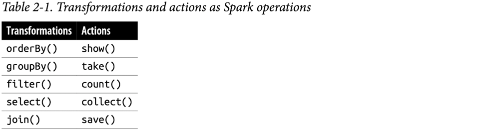
Table 2-1 lists some examples of transformations and actions.
Narrow and Wide Transformations
As noted, transformations are operations that Spark evaluates lazily. A huge advantage of the lazy evaluation scheme is that Spark can inspect your computational query and ascertain how it can optimize it. This optimization can be done by either joining or pipelining some operations and assigning them to a stage or breaking them into stages by determining which operations require a shuffle or exchange of data across clusters.
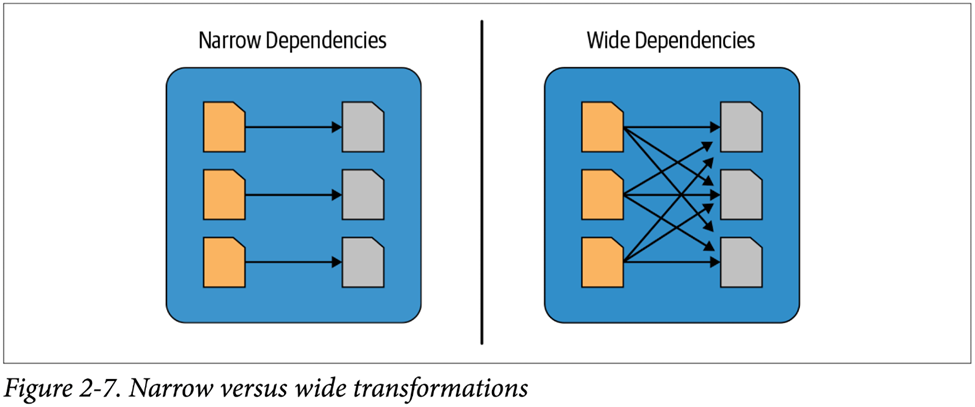
Transformations can be classified as having either narrow dependencies or wide dependencies. Any transformation where a single output partition can be computed from a single input partition is a narrow transformation. For example, in the previous code snippet,filter() and contains() represent narrow transformations because they can operate on a single partition and produce the resulting output partition without any exchange of data.
However, groupBy() or orderBy() instruct Spark to perform wide transformations, where data from other partitions is read in, combined, and written to disk. Since each partition will have its own count of the word that contains the “Spark” word in its row of data, a count (groupBy()) will force a shuffle of data from each of the executor’s partitions across the cluster. In this transformation, orderBy() requires output from other partitions to compute the final aggregation.
Figure 2-7 illustrates the two types of dependencies.
The Spark UI
Spark includes a graphical user interface that you can use to inspect or monitor Spark applications in their various stages of decomposition—that is jobs, stages, and tasks. Depending on how Spark is deployed, the driver launches a web UI, running by default on port 4040, where you can view metrics and details such as:
- A list of scheduler stages and tasks
- A summary of RDD sizes and memory usage
- Information about the environment
- Information about the running executors
- All the Spark SQL queries.
In local mode, you can access this interface at http://<localhost>:4040 in a web browser.
Spark’s Structured APIs
Spark: What’s Underneath an RDD?
The RDD is the most basic abstraction in Spark. There are three vital characteristics associated with an RDD:
- Dependencies
- Partitions (with some locality information)
- Compute function: Partition => Iterator[T]
All three are integral to the simple RDD programming API model upon which all higher-level functionality is constructed. First, a list of dependencies that instructs Spark how an RDD is constructed with its inputs is required. When necessary to reproduce results, Spark can recreate an RDD from these dependencies and replicate operations on it. This characteristic gives RDDs resiliency.
Second, partitions provide Spark the ability to split the work to parallelize computation on partitions across executors. In some cases—for example, reading from HDFS—Spark will use locality information to send work to executors close to the data. That way less data is transmitted over the network.
And finally, an RDD has a compute function that produces an Iterator[T] for the data that will be stored in the RDD.
Structuring Spark
Key Metrics and Benefits
Structure yields several benefits, including better performance and space efficiency across Spark components. We will explore these benefits further when we talk about the use of the DataFrame and Dataset APIs shortly, but for now we’ll concentrate on the other advantages: expressivity, simplicity, composability, and uniformity.
Let’s demonstrate expressivity and composability first, with a simple code snippet. In the following example, we want to aggregate all the ages for each name, group by name, and then average the ages—a common pattern in data analysis and discovery. If we were to use the low-level RDD API for this, the code would look as follows:
# In Python
# Create an RDD of tuples (name, age)
dataRDD = sc.parallelize([("Brooke", 20), ("Denny", 31), ("Jules", 30), ("TD", 35), ("Brooke", 25)])
# Use map and reduceByKey transformations with their lambda
# expressions to aggregate and then compute average

agesRDD = (dataRDD
 .map(lambda x: (x[0], (x[1], 1)))
 .reduceByKey(lambda x, y: (x[0] + y[0], x[1] + y[1]))
 .map(lambda x: (x[0], x[1][0]/x[1][1])))
No one would dispute that this code, which tells Spark how to aggregate keys and compute averages with a string of lambda functions, is cryptic and hard to read. In other words, the code is instructing Spark how to compute the query. It’s completely opaque to Spark, because it doesn’t communicate the intention. Furthermore, the equivalent RDD code in Scala would look very different from the Python code shown here.
By contrast, what if we were to express the same query with high-level DSL operators and the DataFrame API, thereby instructing Spark what to do? Have a look:
# In Python
from pyspark.sql import SparkSession
from pyspark.sql.functions import avg
# Create a DataFrame using SparkSession
spark = (SparkSession
      .builder
      .appName("AuthorsAges")
      .getOrCreate())

# Create a DataFrame
data_df = spark.createDataFrame([("Brooke", 20), ("Denny", 31), ("Jules", 30), ("TD", 35), ("Brooke", 25)], ["name", "age"])

# Group the same names together, aggregate their ages, and compute an average
avg_df = data_df.groupBy("name").agg(avg("age"))

# Show the results of the final execution
avg_df.show()
+------+--------+
|  name|avg(age)|
+------+--------+
|Brooke|    22.5|
| Denny|    31.0|
| Jules|    30.0|
|    TD|    35.0|
+------+--------+
The DataFrame API
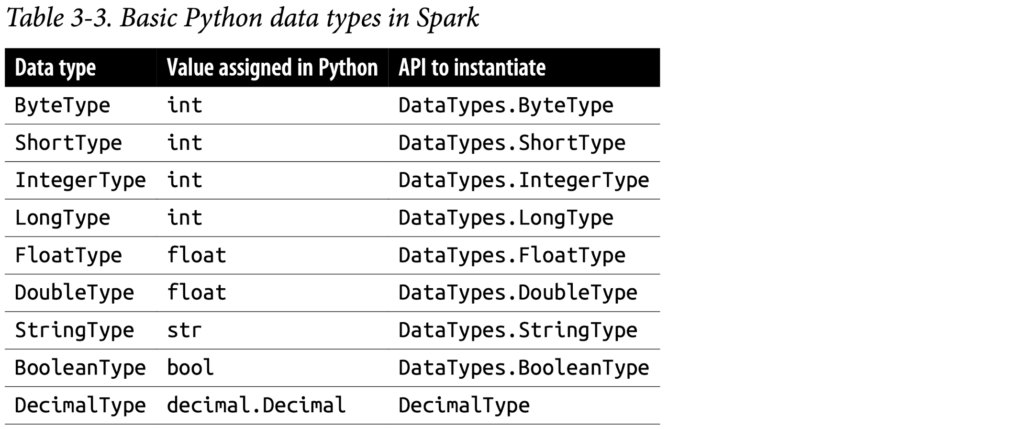
Spark’s Basic Data Types
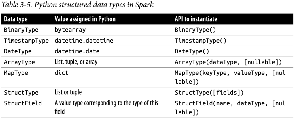
Spark’s Structured and Complex Data Types
Schemas and Creating DataFrames
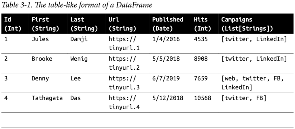
A schema in Spark defines the column names and associated data types for a DataFrame.
Defining a schema up front as opposed to taking a schema-on-read approach offers three benefits:
- You relieve Spark from the onus of inferring data types.
- You prevent Spark from creating a separate job just to read a large portion of your file to ascertain the schema, which for a large data file can be expensive and time-consuming.
- You can detect errors early if data doesn’t match the schema.
So, we encourage you to always define your schema up front whenever you want to read a large file from a data source.
Two ways to define a schema
Spark allows you to define a schema in two ways. One is to define it programmatically, and the other is to employ a Data Definition Language (DDL) string, which is much simpler and easier to read.
To define a schema programmatically for a DataFrame with three named columns, author, title, and pages, you can use the Spark DataFrame API. For example:
# In Python
from pyspark.sql.types import *
schema = StructType([StructField("author", StringType(), False),
      StructField("title", StringType(), False),
      StructField("pages", IntegerType(), False)])

#Defining the same schema using DDL is much simpler:
# In Python
schema = "author STRING, title STRING, pages INT"
You can choose whichever way you like to define a schema.
# define schema by using Spark DataFrame API
schema = StructType([
   StructField("Id", IntegerType(), False),
   StructField("First", StringType(), False),
   StructField("Last", StringType(), False),
   StructField("Url", StringType(), False),
   StructField("Published", StringType(), False),
   StructField("Hits", IntegerType(), False),
   StructField("Campaigns", ArrayType(StringType()), False)])

# define schema by using Definition Language (DDL)
schema = "Id INT, First STRING, Last STRING, Url STRING, Published STRING, Hits INT, Campaigns ARRAY<STRING>"
# avoid reserved word conflict
# schema = "`Id` INT, `First` STRING, `Last` STRING, `Url` STRING, `Published` STRING, `Hits` INT, `Campaigns` ARRAY<STRING>"
Columns and Expressions
Named columns in DataFrames are conceptually similar to named columns in pandas or R DataFrames or in an RDBMS table: they describe a type of field. You can list all the columns by their names, and you can perform operations on their values using relational or computational expressions. In Spark’s supported languages, columns are objects with public methods (represented by the Column type).
You can also use logical or mathematical expressions on columns. For example, you could create a simple expression using expr("columnName * 5") or (expr("columnName - 5") > col(anothercolumnName)), where columnName is a Spark type (integer, string, etc.). expr() is part of the pyspark.sql.functions (Python) and org.apache.spark.sql.functions (Scala) packages. Like any other function in those packages, expr() takes arguments that Spark will parse as an expression, computing the result.
Scala, Java, and Python all have public methods associated with columns. You’ll note that the Spark documentation refers to both col and Column. Column is the name of the object, while col() is a standard built-in function that returns a Column.
Rows
A row in Spark is a generic Row object, containing one or more columns. Each column may be of the same data type (e.g., integer or string), or they can have different types (integer, string, map, array, etc.). Because Row is an object in Spark and an ordered collection of fields, you can instantiate a Row in each of Spark’s supported languages and access its fields by an index starting at 0:
>>> from pyspark.sql import Row
>>> blog_row = Row(6, "Reynold", "Xin", "https://tinyurl.6", 255568, "3/2/2015", ["twitter", "LinkedIn"])
>>> # access using index for individual items
>>> blog_row[1]
'Reynold'
Row objects can be used to create DataFrames if you need them for quick interactivity and exploration:
>>> rows = [Row("Matei Zaharia", "CA"), Row("Reynold Xin", "CA")]
>>> authors_df = spark.createDataFrame(rows, ["Authors", "State"])
>>> authors_df.show()
+-------------+-----+
|      Authors|State|
+-------------+-----+
|Matei Zaharia|   CA|
|  Reynold Xin|   CA|
+-------------+-----+
Common DataFrame Operations
To perform common data operations on DataFrames, you’ll first need to load a Data‐ Frame from a data source that holds your structured data. Spark provides an inter‐ face, DataFrameReader, that enables you to read data into a DataFrame from myriad data sources in formats such as JSON, CSV, Parquet, Text, Avro, ORC, etc. Likewise, to write a DataFrame back to a data source in a particular format, Spark uses DataFrameWriter.
Using DataFrameReader and DataFrameWriter
By defining a schema and use DataFrameReader class and its methods to tell Spark what to do, it’s more efficient to define a schema than have Spark infer it.
inferSchema
If you don’t want to specify the schema, Spark can infer schema from a sample at a lesser cost. For example, you can use the samplingRatio option(under chapter3 directory):
sampleDF = (spark
    .read
    .option("sampleingRatio", 0.001)
    .option("header", True)
    .csv("data/sf-fire-calls.csv"))
The following example shows how to read DataFrame with a schema:
from pyspark.sql.types import *

# Programmatic way to define a schema
fire_schema = StructType([StructField('CallNumber', IntegerType(), True),
                StructField('UnitID', StringType(), True),
                StructField('IncidentNumber', IntegerType(), True),
                StructField('CallType', StringType(), True),
                StructField('CallDate', StringType(), True),
                StructField('WatchDate', StringType(), True),
                StructField('CallFinalDisposition', StringType(), True),
                StructField('AvailableDtTm', StringType(), True),
                StructField('Address', StringType(), True),
                StructField('City', StringType(), True),
                StructField('Zipcode', IntegerType(), True),
                StructField('Battalion', StringType(), True),
                StructField('StationArea', StringType(), True),
                StructField('Box', StringType(), True),
                StructField('OriginalPriority', StringType(), True),
                StructField('Priority', StringType(), True),
                StructField('FinalPriority', IntegerType(), True),
                StructField('ALSUnit', BooleanType(), True),
                StructField('CallTypeGroup', StringType(), True),
                StructField('NumAlarms', IntegerType(), True),
                StructField('UnitType', StringType(), True),
                StructField('UnitSequenceInCallDispatch', IntegerType(), True),
                StructField('FirePreventionDistrict', StringType(), True),
                StructField('SupervisorDistrict', StringType(), True),
                StructField('Neighborhood', StringType(), True),
                StructField('Location', StringType(), True),
                StructField('RowID', StringType(), True),
                StructField('Delay', FloatType(), True)])

fire_df = (spark
 .read
 .csv("data/sf-fire-calls.csv", header=True, schema=fire_schema))
The spark.read.csv() function reads in the CSV file and returns a DataFrame of rows and named columns with the types dictated in the schema.
To write the DataFrame into an external data source in your format of choice, you can use the DataFrameWriter interface. Like DataFrameReader, it supports multiple data sources. Parquet, a popular columnar format, is the default format; it uses snappy compression to compress the data. If the DataFrame is written as Parquet, the schema is preserved as part of the Parquet metadata. In this case, subsequent reads back into a DataFrame do not require you to manually supply a schema.
Saving a DataFrame as a Parquet file or SQL table. A common data operation is to explore and transform your data, and then persist the DataFrame in Parquet format or save it as a SQL table. Persisting a transformed DataFrame is as easy as reading it. For exam‐ ple, to persist the DataFrame we were just working with as a file after reading it you would do the following:
# In Python to save as Parquet files
parquet_path = "..."
fire_df.write.format("parquet").save(parquet_path)
Alternatively, you can save it as a table, which registers metadata with the Hive meta-store (we will cover SQL managed and unmanaged tables, metastores, and Data-Frames in the next chapter):
# In Python to save as a Hive metastore
parquet_table = "..." # name of the table
fire_df.write.format("parquet").saveAsTable(parquet_table)
Transformations and actions
Projections and filters. A projection in relational parlance is a way to return only the rows matching a certain relational condition by using filters. In Spark, projections are done with the select() method, while filters can be expressed using the filter() or where() method. We can use this technique to examine specific aspects of our SF Fire Department data set:
fire_parquet.select("IncidentNumber", "AvailableDtTm", "CallType") \
    .where(col("CallType") != "Medical Incident") \
    .orderBy("IncidentNumber") \
    .show(5, truncate=False)

+--------------+----------------------+-----------------------------+
|IncidentNumber|AvailableDtTm         |CallType                     |
+--------------+----------------------+-----------------------------+
|30636         |04/12/2000 10:18:53 PM|Alarms                       |
|30773         |04/13/2000 10:34:32 AM|Citizen Assist / Service Call|
|30781         |04/13/2000 10:53:48 AM|Alarms                       |
|30840         |04/13/2000 01:39:00 PM|Structure Fire               |
|30942         |04/13/2000 07:42:53 PM|Outside Fire                 |
+--------------+----------------------+-----------------------------+
only showing top 5 rows
What if we want to know how many distinct CallTypes were recorded as the causes of the fire calls? These simple and expressive queries do the job:
(fire_parquet
    .select("CallType")
    .where(col("CallType").isNotNull())
    .agg(countDistinct("CallType").alias("DistinctCallTypes"))
    .show())

+-----------------+
|DistinctCallTypes|
+-----------------+
|               30|
+-----------------+
We can list the distinct call types in the data set using these queries:
# In Python, filter for only distinct non-null CallTypes from all the rows
(fire_parquet
    .select("CallType")
    .where(col("CallType").isNotNull())
    .distinct()
    .show(10, False))
Renaming, adding, and dropping columns. Sometimes you want to rename particular columns for reasons of style or convention, and at other times for readability or brevity. The original column names in the SF Fire Department data set had spaces in them. For example, the column name IncidentNumber was Incident Number. Spaces in column names can be problematic, especially when you want to write or save a DataFrame as a Parquet file (which prohibits this).
By specifying the desired column names in the schema with StructField, as we did, we effectively changed all names in the resulting DataFrame.
Alternatively, you could selectively rename columns with the withColumnRenamed() method. For instance, let’s change the name of our Delay column to ResponseDelayedinMins and take a look at the response times that were longer than five minutes:
# create a new dataframe new_fire_parquet from fire_parquet
# rename "Delay" with "ResponseDelayedinMins" in new_fire_parquet
new_fire_parquet = fire_parquet.withColumnRenamed("Delay",
                                                  "ResponseDelayedinMins")
# select ResponseDelayedinMins > 5 mins
(new_fire_parquet
    .select("ResponseDelayedinMins")
    .where(col("ResponseDelayedinMins") > 5)
    .show(5, False))

+---------------------+
|ResponseDelayedinMins|
+---------------------+
|5.0833335            |
|7.2166667            |
|8.666667             |
|5.7166667            |
|16.016666            |
+---------------------+
only showing top 5 rows
Because DataFrame transformations are immutable, when we rename a column using
withColumnRenamed()we get a new DataFrame while retaining the original with the old column name.
Modifying the contents of a column or its type are common operations during data exploration. In some cases the data is raw or dirty, or its types are not amenable to
Reference:
https://spark.apache.org/docs/latest/rdd-programming-guide.html#actions
https://docs.databricks.com/en/getting-started/dataframes.html
https://sparkbyexamples.com/